Batch ELT from AWS DynamoDB to Snowflake
Tags: snowflake dynamodb aws data elt s3In this article we are going to discuss a new way to batch load your DynamoDB tables directly into Snowflake without proprietary tools. But first…
Why DynamoDB is so popular
AWS DynamoDB is a cloud native NoSQL database service, renowned for its performance and stability. In fact, in a recent AWS blog post about Prime Day, it is claimed it sustained a peak load of 80 million requests per second! Whilst most customers are unlikely to reach that level of sustained throughput, it demonstrates the extent to which the service is designed to scale.
There are a wide range of database options on offer from AWS for different workloads, yet RDS and DynamoDB are by far the most established and with the most mature capabilities to support mainstream and high performance requirements. Both are easily scaled and highly available across multiple availability zones, and even multiple geographical regions. One key differentiator, however is cost model - RDS attracts an hourly pricing model for compute, irrespective of actual demand, whilst DynamoDB charges you only for what you use.
NoSQL databases are often regarded for their schemaless capabilities that - as well as offering flexibility - demand tolerant applications as data structures evolve over time. With AWS DynamoDB in particular, much attention has been paid to single table designs in recent years that optimize read and write patterns in order to effectively allow multiple domains of data within a single table.
Integrating with Data Warehouses
Despite providing flexibility for transactional data users, NoSQL tables often present challenges for analytics teams. It can be difficult to transform semi-structured data to the relational table format found in data warehouses, or make sense of sparse data patterns commonly used in single table designs.
In this article I will to show you how to successfully integrate DynamoDB data with Snowflake, in a cost-effective and cloud native way. We will tackle both the sparse data and semi-structured data challenges, using plain old SQL.
What has changed?
Until very recently, getting bulk data out of AWS DynamoDB typically required the use of either specialised vendor or cloud provider tools (e.g. AWS Data Pipeline), or invest a lot of your own engineering effort to extract the data yourself. In any case, there was no out-of-the-box feature that could dump a DynamoDB table for export, without having a performance, cost or engineering impact.
In November 2020, AWS DynamoDB has released a new feature to export the contents of a table to S3 without performance impact, leveraging Point-In-Time-Recovery (PITR). The cost for this serverless feature is based only on the volume of data that you export, priced at $0.114 per GB in the AWS Sydney region.
This feature - which many would say is long overdue - may be a very welcome feature for those working with data lakes and data warehouses, as it allows for very simple cloud native integrations with your DynamoDB data:
-
Snowflake has excellent support for External Tables that read directly from external stages as well as table hydration from external stages for better query performance
-
Amazon Redshift has good support for integrating data from DynamoDB, however, this latest feature may allow teams leveraging older methods to consolidate and simplify their data access patterns, whilst also eliminating load from their operational tables
At the time of writing, the new export functionality is only available in the AWS DynamoDB V2 console, though it is expected this V2 console will shortly become the default, once it is feature complete. It is also available in SDK libraries and using the AWS Command Line Interface (CLI).
It would be great to see AWS DynamoDB Export evolve to support writing to S3 Access Points instead of only bucket destinations; this would reduce the operational burden and risk of managing cross account S3 access.
What will we learn?
The outcomes of this article are to demonstrate how to:
- Schedule a regular export of your DynamoDB table to S3
- Understand export structures and metadata, and how to use it effectively to work with multiple export copies
- Transform raw data exported from DynamoDB into multiple tables to meet your requirements
The goal is to provide analysts both the data they need in the structure they expect, combined with the visibility and techniques to adapt it over time, as the data changes.
Our Scenario
ⓘ All source code and data files for this blog post are available in the dynamo db export to snowflake repository.
This demonstration will use weather data from Australia’s Bureau of Meteorology (BOM). They have a variety of data available from local weather stations, which is helpful for constructing an example of a single table design based on facts such as:
- Maximum Temperature
- Rainfall
- Solar Exposure
- Generalised Weather records
I have made only basic changes to the (included) original data files to simplify the importing of data into DynamoDB. Data is centered around a YYYY-MM-DD date dimension.
Architecture
The diagram below describes the architecture we will be working with.
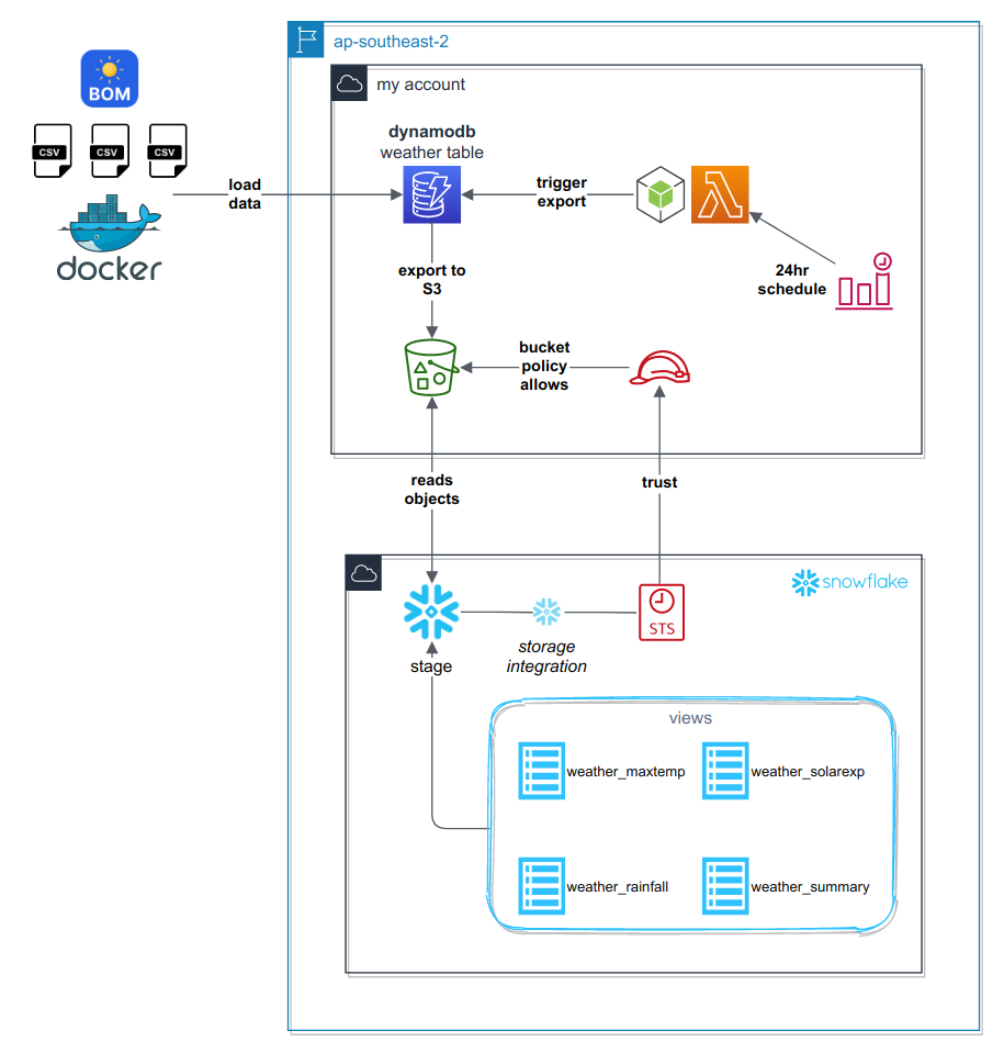
In summary, we:
- Use CDK to create our AWS infrastructure stack:
- AWS DynamoDB table
- Lambda to trigger DynamoDB export
- S3 Storage Bucket
- Snowflake access role
- Import CSV data to DynamoDB using ddbimport
- Create a selection of Snowflake views accessing the staged data directly, to break out our single table design into relational tables
The first two points are covered in the code repository linked above; the rest of this article will focus on accessing the data written by the export process.
Exporting The Data
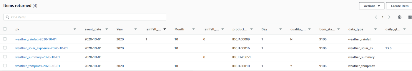
Below is a screenshot of the sparse data from DynamoDB’s new item explorer, to help us visualise the problem we are trying to solve. Note the absence of values in some columns - this is common in single table designs as each row may represent a different kind of data entity.
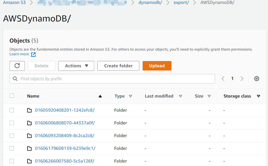
Successive DynamoDB exports to S3
As described in the architecture earlier, we run the DynamoDB export every 24 hours. Observe how each export gets its own folder; it is self contained and stores all of the files managed by an invocation of the export process, as we will see later:
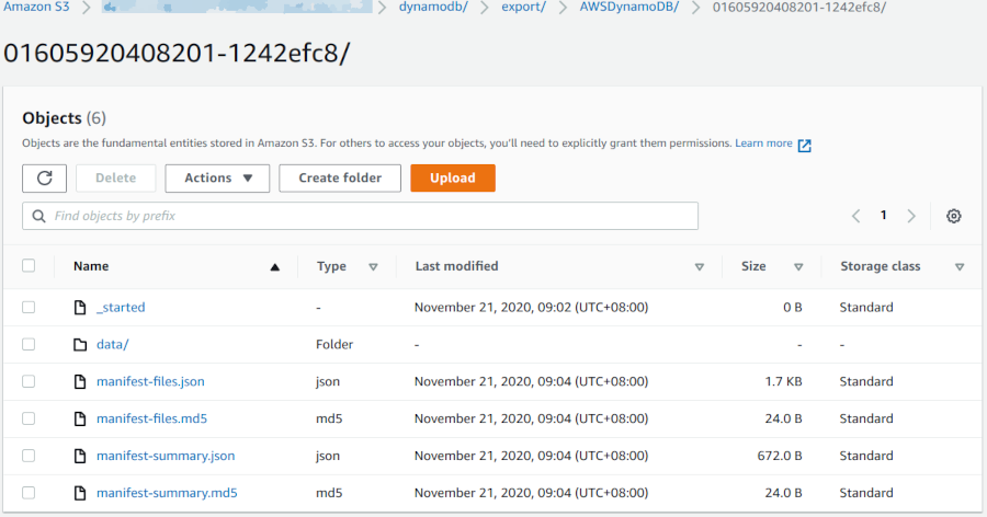
Export Structure
If you have ever enabled inventory reports for one of your S3 buckets, then the pattern followed by DynamoDB Exports will be familiar to you. The following is written for each export performed:
- A manifest file containing a summary of the export process
- A manifest file containing a list of data files containing the DynamoDB table data
- A number of data files containing segments of the DynamoDB table data
Cleaning Up Old Exports
In order to appropriately manage storage used, a lifecycle rule is introduced to delete files older than 3 days from this export folder:
  bucket.addLifecycleRule( {
      enabled: true,
      expiration: cdk.Duration.days(3),
      prefix: exportPrefix,
      id: 'delete-objects-after-3-days'
  });
This will prevent us accruing costs on old exports of the DynamoDB table that we do not need.
Normalizing The Data
Now that we have our DynamoDB table regularly exporting to S3, it’s time to see how we can read that data in Snowflake.
Listing files in the Snowflake stage
If you have set your stage up correctly, you won’t need to use the S3 console to view the exported objects. You can use the following command to show what objects are visible in the Snowflake External Stage:
list @DYNAMODB_SNOWFLAKE_BLOG;
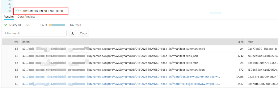
The objects listed in the results should be familiar to you, now that you understand the structure of each DynamoDB table export. How can we find out more about an export, though?
Reading Metadata
Let’s start with the manifest summary: it provides data about the export process.
You can specify a PATTERN when listing files, to show only objects with names matching a particular pattern.
list @DYNAMODB_SNOWFLAKE_BLOG PATTERN=".*manifest-summary\.json$";
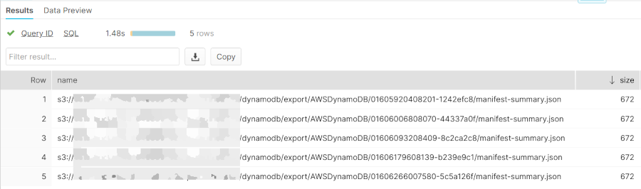
This has provided us the list of manifest summary files only, but how can we see what kind of information these files contain? Let’s just do a SELECT!
Inspecting the manifest summary data with SELECT statements
In Snowflake you can easily run SELECT queries directly against staged data - let’s try the following example:
SELECT $1 FROM @DYNAMODB_SNOWFLAKE_BLOG (PATTERN=> ".*manifest-summary\.json$");
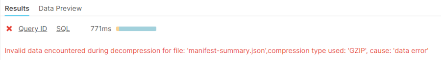
Oh dear! It didn’t work - but it gave us a good clue as to why: DynamoDB Exports write their metadata uncompressed. To address this issue, we need to create a FILE FORMAT that specifies uncompressed data, and then use that file format in our SELECT statement:
CREATE FILE FORMAT PLAINJSON TYPE=JSON COMPRESSION=NONE;
SELECT $1 FROM @DYNAMODB_SNOWFLAKE_BLOG (PATTERN=> ".*manifest-summary\.json$", FILE_FORMAT=>PLAINJSON);
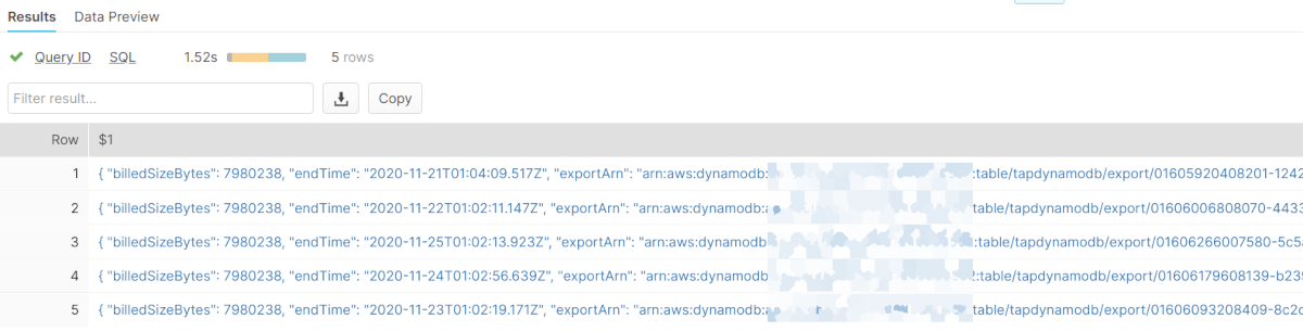
And if you click on the data you can see a prettified preview like this:
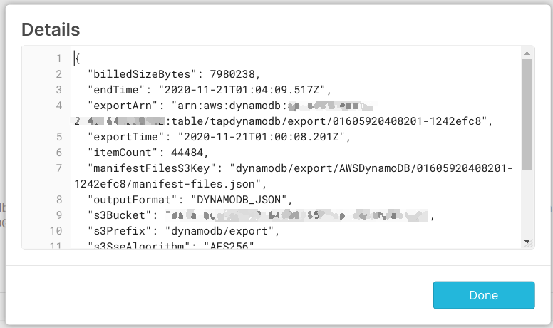
As you can see, there is useful information in there:
- Export Time
- Total number of items exported
- Manifest file key (which we can use to determine the prefix for this specific export)
Take only what you need
So if you noticed before, we use the $1 magic column to return the entire raw data from each row - but you can be much more specific:
select
    -- this returns the s3 object key containing the original data
    metadata$filename as filename,
    SPLIT_PART(filename,'manifest-summary.json',1) as filepath, --
    $1:exportTime::TIMESTAMP_NTZ as exported,
    SPLIT_PART($1:manifestFilesS3Key,'manifest-files.json',1) as dumpPath
  FROM @DYNAMODB_SNOWFLAKE_BLOG/export/AWSDynamoDB (PATTERN=> ".*manifest-summary\.json$", FILE_FORMAT=>PLAINJSON)
  ORDER BY exported DESC LIMIT 1;
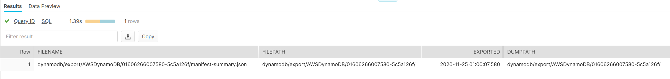
Why is this important? Because it forms the basis of queries that allows us to always work with the latest dynamodb export on S3.
Showing The Latest Data
Now that we have the path to the latest data, here is a query that can provide us the raw data from the latest export:
WITH themanifest AS (
  SELECT
    metadata$filename as filename,
    SPLIT_PART(filename,'manifest-summary.json',1) as filepath,
    $1:exportTime::TIMESTAMP_NTZ as exported,
    SPLIT_PART($1:manifestFilesS3Key,'manifest-files.json',1) as dumpPath
  FROM @DYNAMODB_SNOWFLAKE_BLOG/export/AWSDynamoDB (PATTERN=> ".*manifest-summary*.json", FILE_FORMAT=>PLAINJSON)
  ORDER BY exported DESC LIMIT 1
),
realdata AS (
    SELECT metadata$filename AS datafile,$1 AS datajson FROM @DYNAMODB_SNOWFLAKE_BLOG/export/AWSDynamoDB (PATTERN=> ".*json.gz")
)
select r.datafile,r.datajson from realdata r
join themanifest t on startswith(r.datafile,t.filepath);
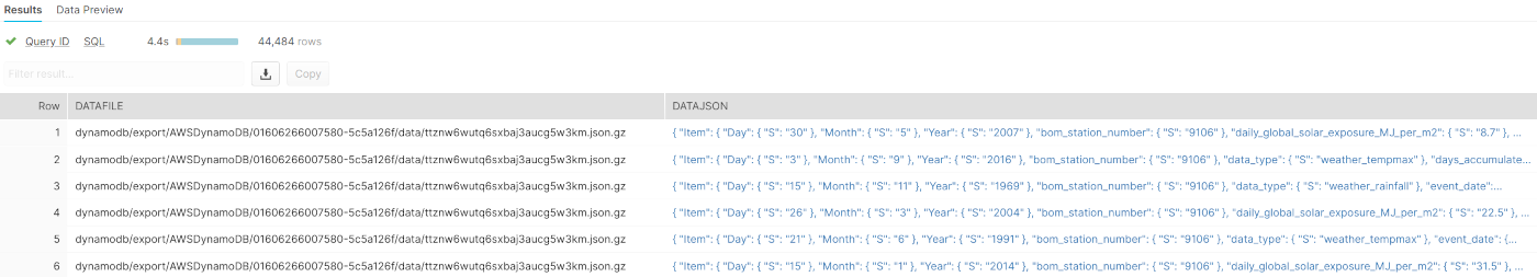
Again, clicking on the data gives a prettified JSON of one of the records:
{
  "Item": {
    "Day": {
      "S": "15"
    },
    "Month": {
      "S": "11"
    },
    "Year": {
      "S": "1969"
    },
    "bom_station_number": {
      "S": "9106"
    },
    "data_type": {
      "S": "weather_rainfall"
    },
    "event_date": {
      "S": "1969-11-15"
    },
    "pk": {
      "S": "weather_rainfall-1969-11-15"
    },
    "product_code": {
      "S": "IDCJAC0009"
    },
    "quality_bool": {
      "S": "Y"
    },
    "rainfall_mm": {
      "S": "0"
    }
  }
}
Iteratively Building Views
At this stage, we can create a view of the raw data by simply prefixing the previous query with something like:
CREATE OR REPLACE VIEW weather_data_raw_latest AS
  ...
;
Everything we do now is going to be an iteration from this view, and the ones that follow.
CREATE OR REPLACE VIEW weather_solar_exposure_raw AS
  SELECT * FROM weather_data_raw_latest WHERE datajson:Item.data_type.S = 'weather_solar_exposure';

CREATE OR REPLACE VIEW weather_rainfall_raw AS
  SELECT * FROM weather_data_raw_latest WHERE datajson:Item.data_type.S = 'weather_rainfall';

CREATE OR REPLACE VIEW weather_tempmax_raw AS
  SELECT * FROM weather_data_raw_latest WHERE datajson:Item.data_type.S = 'weather_tempmax';

CREATE OR REPLACE VIEW weather_summary_raw AS
  SELECT * FROM weather_data_raw_latest WHERE datajson:Item.data_type.S = 'weather_summary';
By creating separate views for each of the different data_type fields, we have essentially normalized the different data entities from the DynamoDB single table design.
Now, let’s create a view to turn the raw data in to a standardised relational form:
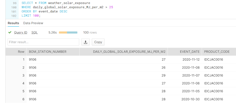
 CREATE OR REPLACE VIEW weather_solar_exposure AS
   SELECT
      datajson:Item.bom_station_number.S::STRING AS bom_station_number,
      datajson:Item.daily_global_solar_exposure_MJ_per_m2.S::NUMBER AS daily_global_solar_exposure_MJ_per_m2,
      datajson:Item.event_date.S::DATE AS event_date,
      datajson:Item.product_code.S::STRING AS product_code
      FROM weather_solar_exposure_raw;
Once views like these are created, data has been transformed to a format suitable for further transformation, or consumption by analytics teams:
Now each data item has its own column, and is of the correct data type. There are a number of advantages to what we have done here:
- additions to DynamoDB row attributes (i.e. schema) will not break these views as they only read what they are looking for
- incorporating new fields is as simple as re-creating the view with the new field specified
- Casting errors or new data attributes can be discovered from the original raw data views
Visualising The Data
Having gone to the trouble to make our data available in Snowflake, we may as well show it off with a small chart.
Let’s make a table that joins the datasets on the event_date field:
CREATE OR REPLACE TABLE materialized_longterm_weather_stats AS
  SELECT
      s.event_date,
      x.daily_global_solar_exposure_MJ_per_m2,
      r.rainfall_mm,
      r.rainfall_period_days,
      t.temp_max_c,
      s.sunshine_hrs,
      s.time_0900_wind_direction,
      s.time_0900_wind_speed_kmh
  FROM weather_summary s
  JOIN weather_rainfall r ON r.event_date=s.event_date
  JOIN weather_solar_exposure x ON x.event_date=s.event_date
  JOIN weather_tempmax t ON t.event_date=s.event_date
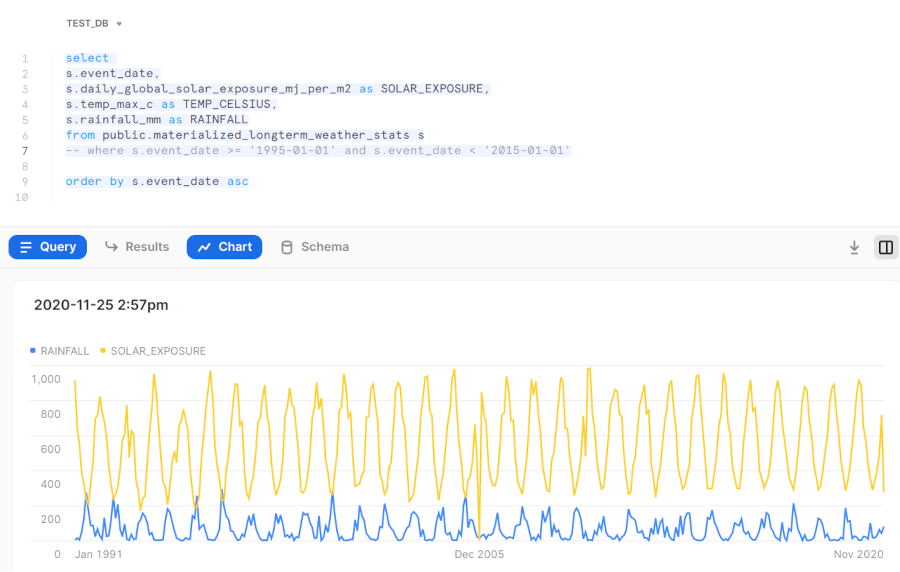
Then simply run a query to visualise the data using Snowflake’s built in data exploration tool, SnowSight:
Performance and DataOps
Performance Considerations: When To Ingest
You will notice in these examples we have not actually ingested any data to Snowflake - we have simply wrapped schema around data that resides on our own S3 bucket.
Snowflake does a great job of caching results from staged data to improve performance, but as soon as your Virtual Warehouse spins down, it will have to re-read that data from S3. This can be both slow and costly, when you have a significant volume of data.
There are a couple of options available
- Ingest the data at some point by running a
COPY INTOor CTAS statement - Create a Materialized View
Both of these will be effective though there are complications and cost considerations with materialized views that often make it simpler to COPY INTO a new table.
DataOps
When working with production systems, you don’t want to be creating views in your SQL workbench.
- Use a DataOps Pipeline to setup and manage your Cloud Data Warehouse
- Materialize and Transform your data with a tool like DBT once it is available in your warehouse
More on that in a future blog post!
Conclusion
In this article we have demonstrated
- How simple exporting DynamoDB tables to S3 can be with the new export feature
- How to work with staged files using Snowflake
- How to normalize semi-structured data into relational views in Snowflake
Get in touch with us at Mechanical Rock to grow your analytics engineering capabilities to the next level!